Chap 8.
°ËÁ¤(Tests)
8.1~2 Hypotheses and Test Procedures
- Def. A test procedure is specified by
1. a test statistic, a function of the sample data on which the decision
(reject H_0 or do not reject H_0) is to be based, and
2. a rejection region, the set of all test statistic values for which
H_0 will be rejected.
The null hypothesis will then be rejected if and only if the observed or
computed test statistic value falls in the rejection region.
- Def.
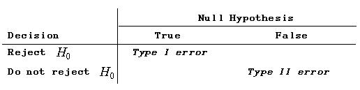
- Prop. Suppose an experiment and a sample size are fixed, and a test
statistic is choosen. Then decreasing the size of the rejection region to obtaion a smaller value of \alpha(Type I error) results in a larger value of \beta(Type II error) for any particular parameter value consistent with H_1.
- Def. The significance level of the test is the maximum value of \alpha (Type I error).
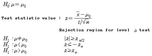
8.3 Tests about a Population Mean
- 8.3.1 Large-Sample
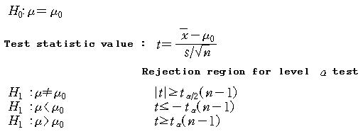
- 8.3.2 Small-Sample
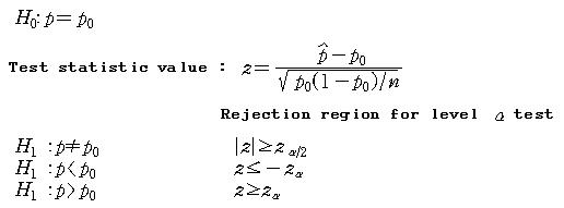
8.4 Tests about a Population Proportion
8.5 Two Sample Tests
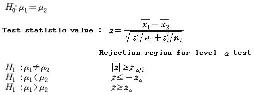
- 8.5.1 Large-Sample
Assumption.
1. X_11, X_12, ..., X_1n1 is a random sample from a population with mewn \mu_1 and unknown variance \sigma_1.
2. X_21, X_22, ..., X_2n2 is a random sample from a population with mewn \mu_2 and unknown variance \sigma_2.
3. The X_1 and X_2 samples are independent of one another.
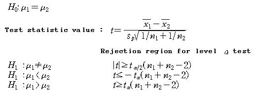
- 8.5.2 Small-Sample
Assumption.
1. Both population are normal, so that X_11, X_12, ..., X_1n1 is a random sample from a normal distribution and so is X_21, X_22, ..., X_2n2 (with the X_1 and X_2 samples are independent of one another.
2. The values of the population variances \sigma_1^2 and sigma_2^2 are equal, so that their comon value can be denoted by \sigma^2.
Def. The polled estimater of the common variance \sigma^2, denoted by
S_p^2 is defined by 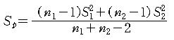 Thm.
Thm. 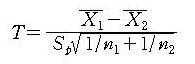 has a t-distribution with m+n-2 degree of freedom. has a t-distribution with m+n-2 degree of freedom.
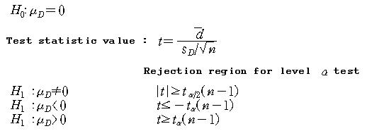
- 8.5.3 Analysis of Paired Data
Assumption.
The data consistes of n independent selected pairs (X_11, X_21), ...(X_1n, X_2n) with E(X_1i)=\mu_1 and E(X_2i)=\mu_2. Let
D_i=X_1i-X_2i so the D_i's are the difference within pairs. Then the D_i's are assumed to be normally distributed with variance
\sigma_D^2.
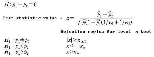
8.6 Tests about a Difference between Population Proportions
Def. The P-value is the smallest level of significance at which H_0 would be rejected when a specified test procedure is used on a given data set. Once the P-value has been determined, the conclusion at any perticular level \alpha results from comparing the P-value to \alpha :
a. P-value <= \alpha = reject H_0 at level \alpha
b. P-value >= \alpha => do not reject H_0 at level \alpha
8.7 Nonparametric Tests
- 8.7.1 Nonparametric methods
In many cases an experimenter does not know the form of the basic distribution and needs statistical techniques which are applicable regardless of the form of the density. These techniques are called nonparametric or distribution-free methods.
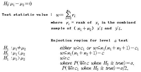
- 8.7.2 Wilcoxon rank sum test
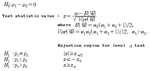
A Normal Approximation for W
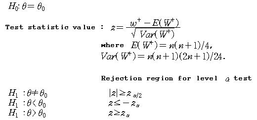
- 8.7.3 Wilcoxon signed rank test
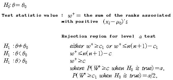
A Large-Sample Approximation
Quiz 8. Email: lbg@kowon.dongseo.a
c.kr
1. Let p denote the true proportion of Budweiser drinkers who can distinguish their beer from Schlitz. If X denote the number of correct identifications in a sample of 100 Bud drinkers and we observe x=57, test H_0:p=0.5 versus H_1:p!=0.5 using a level 0.10 test.
2. Let \mu_1 and \mu_2 denote average tread lives for two different brands of size FR78-15 radial tires. Test H_0:\mu_1-\mu_2=0 versus H_1:\mu_1-\mu_2!=0 at level 0.05 using the following data: n_1=40, \bar x_1=36,500, s_1=2200, n_2 =40, \bar x_2 =33,400,and s_2=1900.
|